
3.3 Strategy: Data-Driven Trading
Key Takeaways
- Many prediction market categories have clean, public data inputs — economic releases, weather measurements, sports statistics — that allow model-based probability estimation
- The edge comes from the gap between the market’s “vibes-based” consensus and your data-derived probability — most traders trade on narrative, not numbers
- You don’t need a PhD or sophisticated machine learning — a simple model using historical base rates and public data often outperforms the crowd
- The framework is: public data → probability estimate → compare vs. market price → trade only when your estimate diverges from the market by more than your TFT
- Data-driven trading is the most teachable and repeatable form of analytical edge
Scope: This module teaches you to build simple, data-driven probability models for prediction markets. It applies the analytical edge framework from Module 3.1 to specific market categories with quantifiable data inputs. It does not cover complex quantitative modeling or machine learning (those are advanced topics for Module 4.1: Building Your Trading System).
The Core Thesis
Most prediction market participants trade on gut feeling, narrative, and recency bias. They watch the news, form an opinion, and bet accordingly. They rarely:
- Look up the historical base rate for the type of event they’re trading
- Build even a simple spreadsheet model
- Systematically compare their estimate to multiple data sources
- Update their views when new data arrives
Meanwhile, many prediction market categories are resolved by objectively measurable outcomes — numbers published by government agencies, weather data, crypto prices, sports results. These outcomes have historical data, trackable precursors, and quantifiable patterns.
If you’re even slightly more systematic than the average trader — which, given the 70% loss rate, is a low bar — you have analytical edge.
Which Markets Are Data-Tradeable?
Not all prediction markets have clean data inputs. Here’s a categorization:
Tier 1: Highly Data-Tradeable (Clean Inputs, Historical Precedent)
| Category | Data Sources | Why It Works |
|---|---|---|
| Economic releases (CPI, GDP, jobs) | BLS, BEA, Fed releases, economic surveys, Cleveland Fed Nowcast, Atlanta Fed GDPNow | These markets resolve on specific numbers with decades of historical data. Models using leading indicators consistently outperform narrative-based trading |
| Federal Reserve decisions | Fed dot plot, futures markets (CME FedWatch), FOMC minutes, inflation data | The Fed is relatively predictable given the right inputs. CME FedWatch already provides a market-implied probability you can compare against |
| Weather / climate | NOAA, NWS, historical weather data, ensemble forecast models | Weather prediction has massive existing infrastructure. GFS/ECMWF model outputs are public and can be directly compared to market-implied probabilities |
| Crypto price thresholds | Bitcoin historical volatility, on-chain metrics, derivatives markets, funding rates | Crypto markets provide real-time, freely accessible data. Historical volatility analysis lets you estimate the probability of price milestones |
Tier 2: Moderately Data-Tradeable (Some Data, Requires Interpretation)
| Category | Data Sources | Limitation |
|---|---|---|
| U.S. elections | Polling aggregates, 538-style models, historical swing data, demographic trends | Polling has known biases; fewer data points per race |
| Sports outcomes | Historical stats, Elo ratings, injury reports, home/away splits | Prediction markets compete with mature sports betting markets that are already highly efficient |
| Corporate milestones | Financial filings, industry data, analyst consensus | Timing-dependent events with significant binary uncertainty |
Tier 3: Narrative-Driven (Minimal Data, High Subjectivity)
| Category | Examples | Why Data Struggles |
|---|---|---|
| Geopolitics | “Will Russia and Ukraine reach a ceasefire?” | Single-actor decisions with no reliable base rate |
| Culture / entertainment | “Will [movie] gross >$1B?” | Limited comparable precedent; viral dynamics are unpredictable |
| Novel events | “Will AI pass [specific test]?” | No historical precedent; expert disagreement dominates |
The strategy implication: Focus your data-driven approach on Tier 1 and Tier 2 markets. Tier 3 markets are better suited to informational edge or fundamental analysis (Module 3.5).
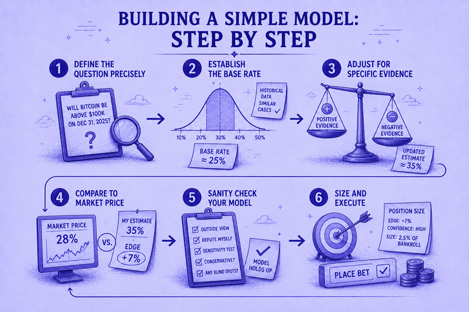
Building a Simple Model: Step by Step
You don’t need to build a neural network. A simple, disciplined framework beats the market more often than you’d expect. Here’s the process:
Step 1: Define the Question Precisely
Before ANY analysis, write down in one sentence exactly what you’re predicting and how it will be resolved.
Good: “Will the BLS unemployment rate for June 2026 (seasonally adjusted, first release) be above 4.5%?” Bad: “Will unemployment go up?”
This seems pedantic, but clarity prevents you from subconsciously shifting your prediction to fit new information — a cognitive bias called “concept creep.”
Step 2: Establish the Base Rate
The base rate is the historical frequency of the outcome you’re predicting. This is the single most powerful tool in your analytical arsenal and is the starting point for every data-driven estimate.
Example: Fed rate decision
Question: “Will the Fed cut rates in June 2026?”
Base rate calculation:
- Since 2000, the FOMC has met 202 times
- Rate cuts occurred at 42 of those meetings (20.8%)
- During periods when inflation was above 3%: 8 cuts out of 78 meetings (10.3%)
- During periods when unemployment was rising and inflation declining: 28 cuts out of 45 meetings (62.2%)
The base rate depends on which conditions match the current situation. Current conditions (April 2026): inflation above 3%, unemployment rising, recent tariff disruptions.
Your base rate selection: The “rising unemployment / declining inflation” base applies best → ~62% base rate for a cut.
💡 Reference class forecasting — choosing the right historical comparison set — is the technique that superforecasters use most consistently and effectively. Philip Tetlock’s research shows it’s the single biggest differentiator between accurate and inaccurate forecasters (Tetlock, Superforecasting, 2015).
Step 3: Adjust for Specific Evidence
The base rate is your starting point. Now adjust it based on evidence specific to this situation:
| Evidence | Direction | Adjustment |
|---|---|---|
| CME FedWatch tool shows 55% probability of a cut (futures market consensus) | Bearish (relative to your 62% base) | Reduces your estimate slightly — but note that CME FedWatch reflects different participants with different information |
| Recent Fed governor speeches emphasize “data dependent” and “patience” | Bearish | Reduces by 5–8%. Hawkish rhetoric typically precedes hold decisions |
| Latest CPI came in below expectations (positive for cuts) | Bullish | Increases by 3–5%. Data-dependent Fed responds to actual data |
| Unemployment ticked up 0.2 points | Bullish | Increases by 5–7%. Dual mandate pressure |
Revised estimate: 62% (base) − 3% (FedWatch caution) − 6% (hawkish speeches) + 4% (CPI surprise) + 6% (unemployment) = 63%
Step 4: Compare to Market Price
Your estimate: 63%. Market price: $0.42 (implying 42%).
Gap: 21 percentage points. This is enormous — far exceeding any reasonable TFT.
But wait: is this gap real, or are you wrong?
Step 5: Sanity Check Your Model
Before trading on a 21-point divergence from the market, challenge your own estimate:
- Have you cherry-picked your base rate class? Try 2–3 different reference classes and see if they converge
- Is the market incorporating information you’re missing? Check news, commentary, and other analytical sources
- Are you anchored to your first estimate? Try starting from the market price and adjusting — do you still end up at 63%?
- Is your sample size adequate? A base rate calculated from 8 data points is much weaker than one from 200
If your estimate survives these challenges — if you genuinely believe the market is that wrong and can articulate why — you have a data-driven trade.
Step 6: Size and Execute
Using the TFT framework from Module 2.3:
- Your edge: 21 percentage points
- Your TFT: ~2% (Polymarket, limit order)
- Net expected edge: ~19%
- Position size: per the 5% rule, max 5% of bankroll
This is a clear, high-conviction trade with a large edge-to-friction ratio. Execute with limit orders, monitor for new information that could change your estimate, and update accordingly.
Worked Example: Weather Market
Market: “Will the high temperature in New York City exceed 95°F on any day in July 2026?”
Step 1 — Precise question: Resolved per NWS Central Park station records.
Step 2 — Base rate: Historical data (1990–2025): At least one 95°F+ day occurred in NYC in July in 22 out of 36 years = 61.1%
Step 3 — Specific evidence:
| Evidence | Direction | Adjustment |
|---|---|---|
| NOAA seasonal forecast: “above-normal temperatures likely for Northeast” | Bullish | +5–8% |
| La Niña conditions developing (historically correlated with warmer Northeast summers) | Bullish | +3–5% |
| GFS 30-day outlook: elevated heat dome probability weeks 2–3 of July | Bullish | +5% |
Revised estimate: 61% + 7% + 4% + 5% = 77%
Step 4 — Market price: $0.55 (implying 55%)
Gap: 22 percentage points.
Step 5 — Sanity check:
- Different base rate using 2000–2025 data: 18/26 = 69.2% (higher, supporting the thesis)
- Climate trend adjustment for warming: significant — NYC has been trending warmer. Using only 2010–2025: 13/16 = 81.3%
- Data sources (NOAA, GFS, La Niña indices) are all publicly available but require domain knowledge to interpret
Assessment: The market is likely underpricing this event because casual traders are estimating temperature probability by “feel” rather than looking at the data. A 22-point gap is large and well-supported.
Step 6 — Trade: Buy Yes at $0.55 on the platform with the best friction profile. Manage position actively — update estimate when July forecast models are published.
Illustrated Example
Common Data Sources for Prediction Market Models
Here’s a practical reference for where to find the data you need:
Economic Markets
| Data Point | Source | URL | Release Schedule |
|---|---|---|---|
| CPI / Inflation | BLS | bls.gov/cpi | Monthly (mid-month) |
| Unemployment | BLS | bls.gov/ces | First Friday monthly |
| GDP | BEA | bea.gov/gdp | Quarterly (advance, preliminary, final) |
| Fed rate probabilities | CME | CME FedWatch | Real-time |
| Inflation nowcast | Cleveland Fed | clevelandfed.org | Real-time |
| GDP nowcast | Atlanta Fed | atlantafed.org/GDPNow | Updated several times/month |
Weather Markets
| Data Point | Source | URL |
|---|---|---|
| Forecasts | NWS / NOAA | weather.gov |
| Historical station data | NOAA Climate | ncdc.noaa.gov |
| Ensemble model output | GFS / ECMWF | Various; tropicaltidbits.com for visualization |
| Seasonal outlooks | NOAA CPC | cpc.ncep.noaa.gov |
Crypto Markets
| Data Point | Source | URL |
|---|---|---|
| Historical prices / volatility | CoinGecko, CoinMarketCap | coingecko.com |
| On-chain metrics | Glassnode, Dune Analytics | dune.com |
| Derivatives data (OI, funding) | Coinglass | coinglass.com |
| Options-implied volatility | Deribit | deribit.com |
Elections / Political
| Data Point | Source | URL |
|---|---|---|
| Polling aggregates | FiveThirtyEight, RCP, Silver Bulletin | 538.com |
| Historical election data | Dave Leip’s Atlas | uselectionatlas.org |
| Approval ratings | Gallup, Morning Consult | gallup.com |
The Data-Driven Trader’s Rules
After building and using models across many markets, these principles emerge:
Rule 1: The Model Is Always Wrong — The Question Is Whether It’s Useful
No model perfectly predicts outcomes. The goal isn’t perfection — it’s being less wrong than the market. If the market is at 42% and the true probability is 63%, your model only needs to get you somewhere between 50% and 80% to be profitable. It doesn’t need to nail 63% exactly.
Rule 2: Base Rates Beat Narratives
When your model says 63% and the news narrative says “there’s no way the Fed cuts,” trust the base rate. Narratives feel compelling but are systematically less accurate than historical frequencies. This is one of the hardest habits to build and one of the most valuable.
Rule 3: Update Continuously, Don’t Anchor
When new data arrives, genuinely update your estimate. Don’t start from your previous estimate and make tiny adjustments (anchoring bias). Start from the base rate, incorporate all current evidence, and re-derive your estimate. If the new estimate is very different from your old one, that’s information — not a mistake.
Rule 4: Trade the Gap, Not the Outcome
You’re not predicting whether the event will happen. You’re predicting whether the market’s probability is wrong. A market at $0.80 for an event you estimate at 85% is a terrible trade — 5% edge barely covers friction. A market at $0.40 for an event you estimate at 63% is an excellent trade — 23% edge, massive cushion.
Trade the size of the gap, not your confidence in the outcome.
Rule 5: Track and Evaluate Your Model’s Accuracy
After every resolved market, record: your estimate, the market’s price, and the actual outcome. Over 50+ trades, calculate your Brier score (the gold-standard metric for forecast accuracy). If your Brier score is consistently better than the market’s implied Brier score, your model is working. If it’s worse, your model is destroying value — and you should stop trading on it.
What You Learned
In this module, you learned:
- Data-driven trading exploits the gap between model-based probability estimates and market prices driven by narrative and intuition
- Three tiers of data-tradeability — Tier 1 (economic, weather, crypto) markets have the cleanest data inputs and strongest edge potential
- A 6-step model-building process — precise question → base rate → evidence adjustment → market comparison → sanity check → execution
- Public data sources for economic, weather, crypto, and political markets provide the raw inputs for your models
- Five rules govern effective data-driven trading: models are useful approximations, base rates beat narratives, continuous updating, trade the gap not the outcome, and track your accuracy
What’s Next
Data gives you analytical edge on markets with clean inputs. But what about markets where the data is ambiguous and the crowd makes systematic errors in judgment? The next module teaches you to exploit documented psychological and structural biases in prediction market pricing.
→ Module 3.4: Systematic Bias Exploitation
🎯 Try This Now: Pick one currently active prediction market in an economic or weather category. Spend 20 minutes building a rough model: (1) Find the historical base rate for the type of outcome being predicted. (2) Identify 3–5 pieces of current evidence that adjust the base rate up or down. (3) Calculate your estimated probability. (4) Compare it to the market price. Is the gap larger than the TFT? If so, you’ve found a potential data-driven trade. Even if you don’t execute it, track the outcome — this is how you calibrate your modeling skills.
Predictionist School is a free educational resource from Predictionist.com. We may earn referral commissions from platforms we recommend — see our disclosure policy for details. This content is for educational purposes only and does not constitute financial advice.